Quickstart

This chapter aims to explain how to use GalaxyChop in general. Here you can see a simple example of

• Reading a galaxy from a file HDF5.

• Explore the attributes of the galaxy.

• Some graphics.

• Aligning and centering the galaxies.

• A simple decomposition.

1. Conceptual overview

By a design decision, and after several prototypes, GalaxyChop was designed in two layers

1. A data representation level, where we defined a class Galaxy which encapsulates all the physical properties useful for the dynamic decomposition.

2. A models level, which understands the Galaxy instances and returns an instance of type Components which represents “to which part of the galaxy each stellar particle corresponds to”.

This first tutorial aims only to give an overview of the project and not to go into too specific details.

Note: About the content

This tutorial is not intended to be a scientific explanation of why and how to perform a dynamic decomposition of galaxies, only to explain the functionalities of GalaxyChop.

2. Creating your first Galaxy

GalaxyChop represents galaxies with a class called galaxychop.Galaxy, which is a collection of gas, dark matter and stars particles each characterized by 3 positions, three velocities, masses and various energies.

To create a Galaxy type object, there are several alternatives, the most useful being to read all the data from a file type HDF5.

So first of all it is necessary to obtain a file with the appropriate content. It is recommended to download this file gal394242.h5 and place it where it is convenient for you.

Note

For convenience we have placed the file gal394242.h5 in the same folder where this tutorial is located.

As a first step it is necessary to import the GalaxChop library, and by simple habit we have taken the practice of assigning to the library the alias gchop.

import galaxychop as gchop

Next we load the file gal394242.h5 using the read_hdf5 function. This will generate an instance of the gchop.Galaxy class.

gal = gchop.read_hdf5("gal394242.h5")
gal

Galaxy(stars=32067, dark_matter=21156, gas=4061, potential=True)

3. Galaxy attributes

Galaxies internally consist of three sets of particles , one for stars, one for dark_matter and one for gas.

All these sets can be accessed, and expose a set of physical properties

For example, if we wanted to access the positions (x, y, and z) of the stellar particles:

gal.stars.x, gal.stars.y, gal.stars.z

(<Quantity [ 0.12017286, -0.01992682, -0.09766993, ..., 15.06957949,
            17.21394372,  9.28556454] kpc>,
 <Quantity [ 1.51520602e-03,  3.25905789e-02, -2.27875536e-02, ...,
             4.52400820e+00, -1.96094867e-01,  1.15665035e+01] kpc>,
 <Quantity [-3.73908514e-02,  5.12012087e-03,  4.66359649e-02, ...,
             1.15501605e+01, -1.40433638e+01,  7.57282498e+00] kpc>)

It can be observed that the positions have units which can be bypassed using the arr_ accessor.

For example if we would like to access the gas masses (m) but without units:

gal.gas.arr_.m

array([2579202.70087197, 1368584.63520184, 1392260.60127839, ...,
        990849.80320185, 1456959.43501778, 1760535.66974588])

The galaxy instances, on the other hand, have useful methods to summarize the data from the three sets, such as summarize the data coming from the three sets, such as angular_momentum_ or gal.kinetic_energy_.

Finally both the arrays and the galaxy in general have methods to create Pandas DataFrames with the particle data.

gal.to_dataframe()

	ptype	ptypev	m	x	y	z	vx	vy	vz	softening	potential	kinetic_energy	total_energy	Jx	Jy	Jz
0	stars	0	5.224283e+05	0.120173	0.001515	-0.037391	10.773575	-6.878906	-20.425400	0.0	-195699.620206	290.293111	-195409.327095	-0.288157	2.051746	-0.842982
1	stars	0	9.745897e+05	-0.019927	0.032591	0.005120	20.282349	8.661957	-7.947495	0.0	-196176.962277	274.782915	-195902.179362	-0.303364	-0.054520	-0.833619
2	stars	0	6.935776e+05	-0.097670	-0.022788	0.046636	-14.897980	6.957092	-10.818886	0.0	-195152.120168	193.699612	-194958.420557	-0.077915	-1.751461	-1.018987
3	stars	0	1.070959e+06	-0.007224	-0.138971	0.176169	-8.665253	-4.337433	5.506927	0.0	-194695.767625	62.113089	-194633.654536	-0.001182	-1.486768	-1.172886
4	stars	0	6.013803e+05	0.095277	0.001167	0.100484	23.508469	-7.842865	-3.754723	0.0	-195703.942688	314.128285	-195389.814402	0.783702	2.719973	-0.774688
...	...	...	...	...	...	...	...	...	...	...	...	...	...	...	...	...
57279	gas	2	1.400046e+06	2.415113	-8.443658	-0.427454	117.975723	-243.209320	31.390686	0.0	-129252.826165	37027.209909	-92225.616256	-369.012963	-126.241204	408.768823
57280	gas	2	1.375867e+06	-4.756847	5.970680	-4.109694	-136.718105	232.501099	-56.024063	0.0	-129835.893336	37943.648417	-91892.244919	621.006707	295.371727	-289.672123
57281	gas	2	9.908498e+05	-9.376904	-1.965296	-0.563573	-188.311616	31.467773	179.615128	0.0	-132966.102621	34356.539847	-98609.562774	-335.262575	1790.361085	-665.158420
57282	gas	2	1.456959e+06	-6.880090	0.314529	-6.284694	-261.390251	69.243408	-137.456593	0.0	-132205.106762	46006.913910	-86198.192853	391.939479	697.043885	-394.186002
57283	gas	2	1.760536e+06	-7.371887	2.670409	-6.167000	-282.899384	138.414307	-134.297680	0.0	-127609.955549	58613.224160	-68996.731389	494.971200	754.613090	-264.917457

57284 rows × 16 columns

4. Visualizing the galaxy

Galaxies have a set of utilities to visualize on the one hand all the particles in the real space; and on the other hand only the stellar ones in the circularity space.

Thus a good summary plot of a galaxy can be made with the command:

gal.plot()

<seaborn.axisgrid.PairGrid at 0x7f288e98baf0>

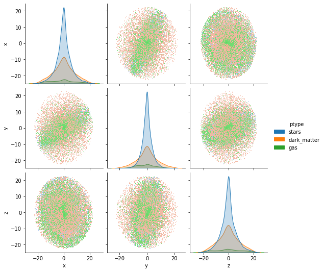
At this point we observe in the graph that the galaxy is neither centered nor aligned, this can be validated with:

print("Centered:", gchop.is_centered(gal))
print("Aligned:", gchop.is_star_aligned(gal))

Centered: False
Aligned: False

To correct this GalaxyChop has the center() and star_align() functions which can be composed as follows

gal = gchop.star_align(gchop.center(gal))
print("Centered:", gchop.is_centered(gal))
print("Aligned:", gchop.is_star_aligned(gal))

Centered: True
Aligned: True

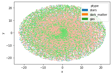
We can also visualize the result, for example by comparing the positions at x and y, highlighting according to the particle type.

gal.plot.hist("x", "y", labels="ptype")

<AxesSubplot:xlabel='x', ylabel='y'>

5. Chop the galaxy

Finally, let’s decompose a galaxy into its parts. The package offers several decomposition models as well as a framework to create new methods. methods.

For didactic reasons we will stick to the method presented in the work of Abadi et al.(2003), which in the context of GalaxyChop is called JHistogram.

The analysis can be summarized in the following steps

1. Instantiate the decomposer

decomp = gchop.models.JThreshold()

2. Decompose the galaxy into components

components = decomp.decompose(gal)
components

Components(57284, labels=[ 0.  1. nan], probabilities=False)

As you can see by the labels [0 1 nan] the decomposer found two components (0 and 1) and could not classify at least one particle, so the meaning of nan for Galaxychop can be understood as “I don’t know what to do with this particle”.

Another detail to take into account is that GalaxyChop decomposes galaxies, but since the dynamic decomposition for gas and dark matter is not defined, it assigns the label nan to all particles.

Finally, it is seen that this classifier does not provide probabilities of particle belonging to a label as it does particle to a label as does GaussianMixture.

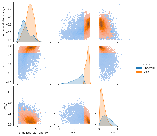
3. Now we can see the division of the particles in the circularity space.

gal.plot.circ_pairplot(labels=components, lmap={0: "Spheroid", 1: "Disk"})

<seaborn.axisgrid.PairGrid at 0x7f288576a7c0>

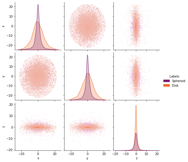
or in the real space

gal.plot.pairplot(
    labels=components,
    lmap={0: "Spheroid", 1: "Disk"},
    palette="inferno",
)

<seaborn.axisgrid.PairGrid at 0x7f287e964fa0>

Finally you can convert the entire components into a Dataframe

components.to_dataframe()

	labels	ptypes
0	0.0	stars
1	0.0	stars
2	0.0	stars
3	0.0	stars
4	0.0	stars
...	...	...
57279	NaN	gas
57280	NaN	gas
57281	NaN	gas
57282	NaN	gas
57283	NaN	gas

57284 rows × 2 columns